GNSS antennas are designed to suppress the reflected signal before it reaches the antenna. However, some of the reflected signals interfere with the direct signal, leading to a multipath effect in the GNSS observations. Reflected signals are used in many remote sensing applications. The determination of sea level variations is also included in these applications.
Cansu Beşel, a researcher from Karadeniz Technical University, Department of Geomatics Engineering, Turkey, has recently published a paper determining the sea level variations along the Turkish Mediterranean coast using GNSS-R. For this purpose, the monitoring sea level was assessed by using the MERS station located in Erdemli, Mersin, on the Mediterranean coast of Turkey. In this paper, the dominant multipath frequency in the SNR data is derived with two methods presented: the Lomb-Scargle periodogram (LSP) and the LSP with the Moving Average (MA) filtering.
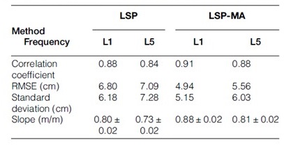
Time series of the sea level heights derived from LSP analysis can contain irregular variations. Thus, reasonable results cannot be generated for sea level heights. This study uses the moving average filtering method to eliminate these irregular variations. First, GNSS-R sea level heights were retrieved using the LSP method. Then, these results were used as input data in the MA filtering method and reconstruct the sea level heights. The GNSS-derived sea level observations were computed by the LSP and LSP with MA method and were compared with nearby tide gauge records. Figure below shows the comparison of GNSS-R retrievals and tide gauge records using LSP and LSP with MA method.
Sea level at MERS station estimated from GNSS-R and sea level recorded by Erdemli tide gauge. GPS- L1 signal is shown in the top, GPS-L5 signal is shown in the bottom.
LSP with MA method indicated improvement in GNSS-R derived sea level, decreasing the RMSE and standard deviation. The results of the LSP and the LSP with MA method are presented in the table below. The GNSS-R-derived sea level observations and sea level records from a nearby tide gauge show similar trends. It should be noted that the performance of the SNR data at the MERS site could be improved with a higher sampling rate and different quality control metrics.
Precipitation detection over ocean using various radar remote sensing techniques have been fully understood and tested for several decades. But in terms of GNSS Reflectometry, researchers had been skeptical about its potential as a rain detector. Recently, a groundbreaking paperhas been published by Dr. Milad Asgarimehr and his colleagues addressing this question cropping up in another paper published three years ago.
Having done his Ph.D. with Technische Universität Berlin, Berlin, Germany, Milad is currently doing his postdoctoral research on improving GNSS-R observations with AI at the German Research Centre for Geosciences (GFZ). Although the GNSS-R capability of rain detection had been doubted at the beginning, Milad’s recent study suggested that precipitation affects the power of reflected GNSS signals, which can be critical in GNSS-R experiments as we prefer to seek for unaffected data.
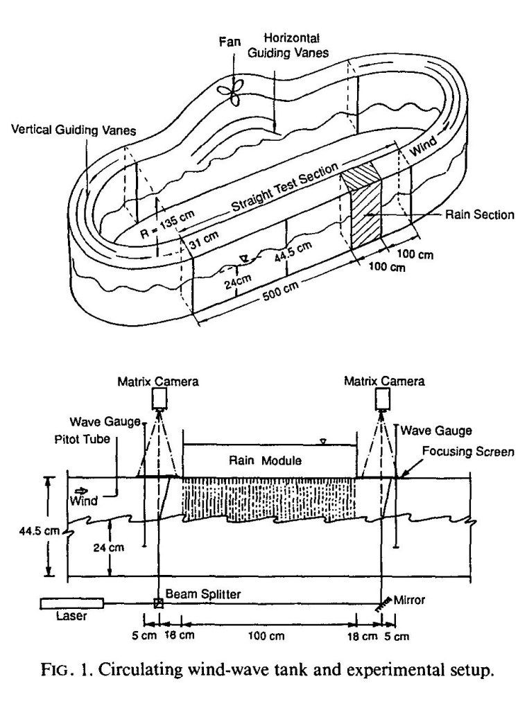
Regardless of microwave remote sensing, the effect of rain on ocean waves and currents has been simulated in laboratory experiments. As an example, this study designed a circulating wind-wave tank to simulate rain drops effects on ocean surface waves showing that ring waves caused by rain drops can amplify the surface roughness at centimetre scales although it can attenuate gravity waves over ocean surfaces. However, these laboratory studies could not fully explain the mechanism of rain effects on ocean surfaces in real environment.
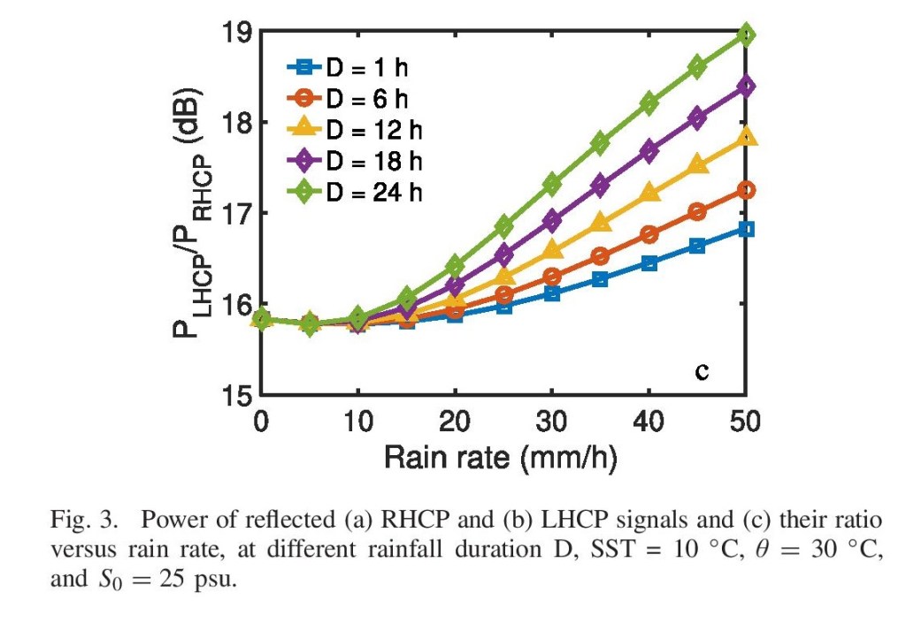
In this recent study, Milad tested the rain effect by analyzing polarimetric GNSS observation at a GFZ coastal GNSS-R station at Onsala Space Observatory in Sweden equipped with two side-looking antennas at two different polarizations (RHCP and LHCP). Among multiple results obtained from this experiment, including sea surface salinity changes due to rain events, the key one was discerning rain drops in the power of RHCP and LHCP reflections over a calm sea. Analyzing the I/Q components of the reflected signals, authors has shown that the received signal power at a low-wind-speed condition (<5 m/s) is reduced due to the diffuse scattering caused by rain-drop-made ring-waves over sea surface.
Reviewing this paper, I came up with this question if we could study ice bottom roughness using GNSS-R tools as either a ground-based or a satellite payload sensor. As discussed in a previous post, mid-winter warm temperature may cause changes in ice roughness, and this variation can be significant enough to be discerned by reflected GNSS signals. In addition, the water underneath the ice is so calm that satisfies the weak diffuse scattering regime condition, similar to the low-wind-speed condition Milad suggested in his paper. To see if GNSS-R has the potential to be used as a roughness indicator, the same steps can be taken as Milad has; however, a very big challenge is ahead of us in lake ice remote sensing: multi-layer scattering! In most GNSS-R studies, the reflection is assumed to be from a single reflective layer, e.g, sea water surface, but in lake ice, as shown in my master’s thesis, there are usually multiple reflective layers unless we experience consecutive days with a cold temperature so we can neglect undesired L-band reflections from layers rather than the ice-water interface.
To be specific, our Haliburton experience, which has been explained in Chapter 4 of my master’s thesis, clearly reflects the temperature effect in the power retrieval process (see this post). But aside from the temperature effect, Milad’s paper shows that GNSS-R is able to detect topography changes in small amplitudes. In other words, if the temperature is cold enough to avoid wet layers, ice bottom roughness may change the power of reflected signals as GNSS-R has well shown the potential to discern the rain-caused roughness in the order of ~5 to 50 mm. However, the other big challenge we may face is ancillary data about real ice bottom roughness, which seemingly necessitates another lengthy fieldwork. Dr. Grant Gunn has recently conducted a research on freshwater ice roughness and capacity (will be bulished by Jun 2021) summerizing multiple methods of ice roughness retrieval and explaining in-situ measurements they have done for this purpose in the Straits of Mackinac region of the Great Lakes between Michigan’s upper and lower peninsulas.
“Why talk to others when you can talk to yourself?” This is how Clara Chew captioned her fantastic YouTube video in LinkedIn to start suggesting a spatial interpolation method for CYGNSS data.
First of all, I should say what a great idea form one of my most inspiring and favorite researchers. Establishing a YouTube channel to talk to ourselves about GNSS reflectometry is what we’d need, and to be honest, that’s the main encouragement for myself to kick off this website. Although I am currently the only writer here, but this platform is going to become an online magazine for GNSS-R researchers to freely read and write others’ opinions. It’s yet to be widely advertised, but the core idea is the same: let’s just talk to ourselves : )
About the video, let’s start from the end; this method is not going to be used for every application. “If you are trying to do some sort of analysis where you need exact knowledge of reflectivity at a certain point,” Clara clarifies “you might not want to use this method”. It sounds very true for my current research focusing on Qinghai Lake, Tibet Plateau, where I restricted Fresnel Zones to only the central region of the lake to make sure that I am not receiving reflections from the surrounding lands or even the shore lines. So, no interpolation is required at any level. But aside from the Qinghai’s research, it’s been a few months that I’ve been thinking about expanding my CYGNSS explorations to a wider region, say central desert of Iran, and meanwhile, one of my greatest concerns has been how to do data interpolation over a large area. Clara has also mentioned it somewhere in her video that “trust me, it won’t be too frustrating”, but it is for me :)) because I haven’t started yet.
But when I’m saying my concern is on how to do it, I wouldn’t say that choosing the interpolation method is not a big concern, as it really is, but it is not the biggest issue for me, because I had practiced a method years ago. The story took place in 2013-2015, when I was working on geodynamics of the Earth, and my specific research at that time was calculating strain tensors. I found out that routine methods for interpolating crustal movement values, e.g. IDW and Spline, are way off the road. I spent couple of months on that, and realized that “deterministic interpolation methods” do not perfectly work for those problems which require “geo-statistical interpolation methods”, such as Kriging. That was the point.
In short, despite deterministic methods which only consider distance as the effective parameter in weighting procedure, geo-statistical interpolation methods also take the correlation into account as a weighting function. This is exactly what Clara suggested: “correlation coefficients“. In Kriging, for example, a covariance matrix is created among node points based on statistical constraints, and then, that matrix plays a key role in establishing the weighting function. The same idea can be seen in another powerful interpolation method called Least-Square Collocation, which is widely used in geoid problems and potential field anomaly interpolations.
I employed Ordinary and Universal Kriging interpolation techniques for estimating strain matrix components, and improved the accuracy up to 70%. As Clara has remained the discussion open at the end of her video, I would invite her to a collaboration in order to explore the ability of geo-statistical methods of interpolation in CYGNSS cases.
Our poster was presented on the first IAG’s conference-workshop on “Geodesy for Climate Research” which is currently (March 29-31, 2021) being held online. The idea of this poster, as can be understood from the title, was on examining the temperature effect on GNSS reflectometry over lake ice.
During the freezing season of 2019-2020, a GNSS-R experiment was conducted at a mid-latitude frozen lake called MacDonald Lake to examine the ability of GNSS interferometric reflectometry for lake ice remote sensing. The initial plan was analyzing GPS signals reflected from the lake to monitor ice formation and generate an ice thickness chart for those dates. However, due to natural features of temperate lake ice covers, such as warm temperatures and mid-winter melt/refreeze events, ice-thickness estimation using GNSS-R was not as straightforward as other routine GNSS altimetry applications conducted before over snow fields or sea surfaces. Meanwhile, the footprints of other lake ice features, such as slush and wet snow, were appeared on the recorded GNSS-R data.
Among those side-parameters, temperature was chosen for this poster. One may think that, by the word temperature effect, I am talking about the tropospheric effects on GNSS signals, such as delay and bending effects, which do matter and have been evaluated for near surface GNSS-R receivers, but I do not mean that. Except for the tropospheric effect, and also the electrical aspects of GNSS receivers, temperature does not directly impact reflected GNSS signals. The point is that temperature causes mid-winter melt/refreeze events in lake ice and, by implication, changes the roughness patterns of reflective layers. Therefore, roughness is the key driver affecting the reflected signals, which is itself affected by temperature variations.
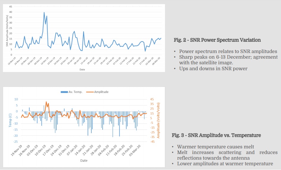
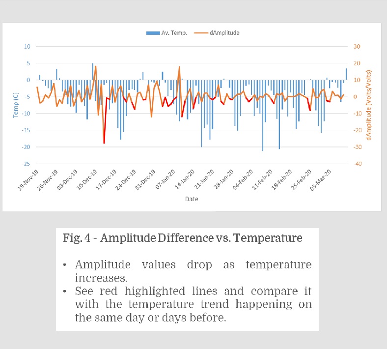
To be specific, for this experiment, we used the SNR-analysis approach in which daily SNR files were extracted and their frequency were calculated to retrieve the antenna heights above reflective surfaces, which could be the ice-water interface, slush layers, or top of the wet snow pack. More details can be found in Chapters 2 and 4 of my master’s thesis. Meanwhile, the power spectrum related to those frequencies showed to be varying over the time, i.e., as shown in Fig 2 in the poster, the SNR amplitude values were not necessarily the same among different dates. Plotting this ups and downs against daily temperatures, as shown in Fig 3 of the poster, we see a harmony, which can be meaningful.
Around Dec 10-15, the freeze-up event happened and a large spike appeared; afterwards, the SNR power values dwindled to almost a third or less and that sharp spike never showed up again. This might be explained by saying when a thin layer of ice appears at the beginning of the freeze-up period, a calm ice/water surface appears whose roughness is much less than that of the lake water in the absence of the ice just before the freeze-up. So, it makes sense if we say the surface became very reflective and a huge reflection happened towards the GNSS antenna. This explanation has been also used in previous GNSS reflectometry studies, e.g. Qingyun Yan‘s research items on sea ice remote sensing through investigating DDMs. However, this reflectivity does not last for a long time as roughness conditions of the reflective layer(s) changes due to lake ice evolution, precipitation, wet layers appearance, and so on. Nevertheless, an agreement can be seen between temperature variations and SNR spectrum vales, so that when the temperature is close to or above zero, small jumps can be seen in SNR amplitudes. To better illustrate this co-variation, Fig 4 is plotted in the poster to illustrate SNR jumps against temperature.
As shown there, when temperature rises, red lines appear in “dAmplitude” values meaning that there are downward jumps in the SNR spectrum. It is not always true, but it mostly happens. Besides, a delay may be seen in this co-variability, which may be because of the time needed for melt/refreeze events to proceed. Meanwhile, one of our co-authors, Justin, who is currently doing his Ph.D. on lake ice remote sensing with the University of Waterloo, raised questions about my explanation and said “as shown in Fig 3, an increase in temperature mostly causes an increase in SNR amplitudes”. This statement retracts from the validity of the poster idea. “This is also agree with what we have in the physics of remote sensing”, Justin added “where wet layers appeared due to melt event leads to a higher dielectric constant and results in stronger returns”.
Justin’s criticism elicited my response by referring to bi-static radar properties where receivers and transmitters are not collocated; so an increase in dielectric constant does not necessarily bring about an increase in reflection strength towards the antenna. Instead, roughness has the main effect even if it happens at very small scales, as recently shown in Milad Asgarimehr‘s studies on the effect of small-scale roughness changes on GNSS signals reflected off oceans. However, my explanation may not look satisfying as those warm days are only some occasions; so, significant trends yet to be derived from this new idea with a short time series. It should be noted that Justin justly mentioned to the refreeze event as a concomitant of the melt event and its significant impact on the roughness, because I hadn’t included the refreeze event and only mentioned to the melt event in the first draft of the poster.
The bottom line is that climate change may show it’s effects on GNSS signals reflected off frozen lakes; however, further investigations are required for achieving to a firm conclusion. Longer time series may be required for future studies to extract more meaningful trends and correlations.
Two papers were recently published focusing on the effect of surface elevation on terrestrial reflected GNSS signals; one is analyzing the effect of surface roughness as small-scale elevation changes on an air-borne GNSS-reflectometry platform, while the other is taking large-scale elevation changes into account and introducing an on-board constraint for DDMs produced by space-borne GNSS-R systems.
Joan, a Ph.D. candidate with Universitat Politècnica de Catalunya, Spain, working on GNSS-Reflectometry published his most recent paper on Feb 22, 2021, discussing their air-borne GNSS-R experience for retrieving soil moisture. The focus of this paper is solving non-linear reflectivity equation using an artificial neural network based algorithm instead of considering all effective variables and solving the functional model. The rationale behind this strategy is amazing; if any of the variables in the reflectivity model was estimated incorrectly, the soil moisture values retrievals could be dead wrong. For example, the impact of soil moisture on the reflectivity could be as high as ~17 dB, while the surface roughness could change the reflectivity by itself up to ~18 dB over a surface with only 4 cm RMSE in surface elevation changes. Even changes more than this value can be simply seen in farmlands. The effect of surface roughness on reflectivity can be seen in the Figure 9 of the paper.
Except for the surface roughness, other factors affecting the incoherent scattering, as the authors say, are those related to vegetation whose modelling with existing indices, e.g., VOD and NDVI, looks easier than that of the surface roughness effect. In addition, changes in the GPS integration time is an effective factor on the reflectivity, so that the higher the effective integration time is set, the less sensitive to surface roughness are the reflections. However, a bias in reflectivity in the along-track direction is introduced requiring a correction before the NDVI measurements. Moreover, the authors has used statistical metrics of the reflectivity itself, e.g. standard deviation, instead of too much ancillary data as a control for their machine learning approach, and addressed a question regarding the relationship between these statistics and the surface roughness.
The question that I would like to ask Joan and the team is about the relevance of averaging over multiple foot prints. In other words, if we conduct a multi-pass flight (rather than a single-pass one) and define the flight path so that we have multiple specular points over each specific known terrestrial point, is there anyway to cancel or reduce the impact of this small-scale topographies on the reflectivity? This suggestion may be applied in drone-based GNSS-R sensors with high maneuver abilities over farmlands. This idea has been tested and featured in summer 2020 and can be found here.
The second research, which was released on March 9, has been published by Lucinda, who is doing her Ph.D. with the University of Surrey, UK, and investigating the use of GNSS-R for Earth observations. Despite the first paper, this paper focuses on the effect of large-scale surface elevation changes on DDMs obtained from TDS-1 GNSS-R observations and their impact on soil moisture estimation. The authors mentioned that the Earth is approximated by a quasi-spherical model to predict specular points (SP) positions. Although this approximation works good for ocean scatterometry as ocean surface represents a quasi-sphere with small height anomalies smaller than 100 m, it would not always be sufficient for land sensing purposes as terrestrial topography impacts the SPs positioning accuracy. Looking at DDMs obtain from SPs with different altitude, one may see a movement in the peak-power location due to this inconsistency between the quasi-spherical model and real surface topography. An example is shown by the authors in the first figure of their paper.
The authors aimed to establish an on-board algorithm to capture signals reflected from any SP at any surface elevation, which is a huge advance comparing to similar recent studies addressing only limited special conditions. This algorithm is to be tested on a GNSS-R SSTL payload, called ToD-1. The key of the proposed algorithm is transforming SPs locations from a geodetic frame to a local geodetic frame, correcting the height element using a proper DEM, and reversely transforming the SPs coordinates to the initial geodetic frame. Results from tests operated on TDS-1 data were promising; the algorithm performed stunning at re-centering DDMs peak-powers.
Although this paper appears really inspiring for me, as I’m investigating some CYGNSS potential for land observation, a question cropped up regarding the peak-power movements among multiple DDMs assigned to one location but recorded at different times. To be more specific, a clear movement can be seen among DDMs obtained from the central area of Qinghai Lake, Tibet Plato, at different epochs. Three following figures are DDMs related to Oct 7, Oct 29, and Nov 14, 2020, respectively, obtained from CYGNSS micro-satellites; it’s obvious that there are movements along delay axis.
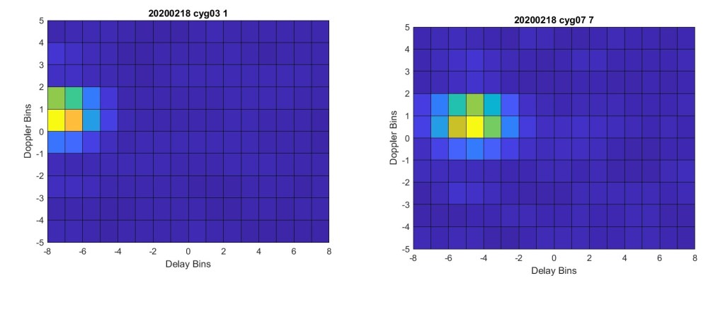
Surprisingly, on Feb 18, 2020, DDMs obtained from two different CYGNSS vehicle have shown different shifts in peak-power from the DDM centre.
Comparing these DDMs to each other, I wonder if there are any other effective factors, rather than topography, on peak-power shifts from/towards the DDM centre. The reason that I ask this question is that Qinghai Lake’s surface can be assumed flat, and in the presence of lake ice, the ice is not so thick to cause a significant topographical movement in the lake surface height.
Space platforms for GNSS Reflectometry back to 33 years ago.
In 1897, Marconi Company was founded in Chelmsford, England, as the division of defense industry and businesses of its mother: General Electric Company. However, it’s known today as BAE Systems plc, a British aerosystem and defense company with its headquarter based in London and Farnborough, UK. By the end of World War II, Marconi put more focus on radio propagation and its application in radio telegraphy. In 1988, David Hall and Ralph Cordey from the Marconi Space Systems and Marconi Research Centre, respectively, discussed the multistatic scatterometry concept using GPSS signals. Apparently, GPS was used to be called GPSS at that time. It’s interesting to know that Hall and Cordey compared GPS signals features, such as code sequence length and transmitted power, with monostatic criteria of ERS-1 (the first remote sensing mission lunched by ESA) and argued that although GPS reflectometry is conceptually possible, the design of GPS at that time are incapable of solving ambiguities due to the weakness of transmitter power output. We’ll talk about GPS transmitter power later.
In 1991, a french alpha-jet aircraft manufactured by Dassault Electronique Company, conducted an experiment to test GPS receivers ability for real time positioning. Flying at low elevation over Atlantic Sea, the aircraft found the positioning solution disturbed due to multipath effect, which meant that reflected GPS signals could be tracked. Dassault Electronique conducted another study to describe and model multipath signals by defining a flight pattern in which direct and reflected GPS signals could be separately recorded. Jean-Claude Auber and co-authors documented this experiment and characterized GPS multipath over land and sea in 1994. They did this to avoid multipath as a harmful phenomenon in positioning, but you know, one’s signal is another one’s noise, and this research led to introducing a new remote sensing tool: GPS-Reflectometry.
In 1993, Manuel Martín-Neira, who had recently been awarded a fellowship to study on microwave radiometry at ESA, developed the concept of Passive Reflectometry and Interferometric System (PARIS) as a tool for ocean altimetry. This new concept opened a new gate to perform altimetry experiments along directions other than nadir, which was the only possible direction for altimetry at that time, by collecting reflected GPS signals off the ocean from various directions. Explaining the geometry and instrumentation of PARIS, Dr. Martín-Neira explained how one can reach to the vertical accuracy of 70 cm with GPS altimetry. He, for the first time, depicted the patterns of iso-range and iso-Doppler curves formed in GPS altimetry, and how they differ from those in the monostatic SAR case, i.e., how the orientation of iso-range and -Doppler curves may differ from each other depending on the direction of GPS satellites and receiver velocity. Considering patenting of this idea as a turning point, Dr. Martín-Neira has said: “Having had this idea, which was not particularly well received, the proposal by ESA’s Patents Group to patent it made all the difference. It gave me a feeling of confidence, that somebody else at least saw the potential of this idea – and the rest is history”
Finally, five years later, Jet Propulsion Laboratory reported that GPS reflections have been observed, for the first time, by the Space-borne Imaging Radar-C (SIR-C) aboard the shuttle. That was the first space-borne observation of GPS signals reflected from the Earth, the Pacific Ocean, giving insights into the expected SNR at the receiver.